An illustration of permutation testing in GWAS
Without loss of generality, consider a genetic association study with 10 SNPs weakly associated with a quantitative trait. We would like to assess the significance of these SNPs after multiple testing correction.
10 SNPs are independent
Let’s simulate the genotype data first, assuming the SNPs are independent, and a sample size of $N=1,000$ unrelated individuals,
# set random seed
set.seed(999)
# Sample from a multivariate normal distribution for SNP matrix X, as if the SNP data has been normalized,

n <- 1000
p <- 10
R <- diag(p)
mu <- rep(0,p)
X <- MASS::mvrnorm(n, mu = mu, Sigma = R)
Now we simulate the 10 SNP effects, assuming 0.5% heritability in each SNP,
sigma2 <- 0.005
b <- rnorm(p, 0, sqrt(sigma2))
then simulate phenotype vector $y$ as $y = Xb + e$ where $e$ is a vector of $N(0, \sqrt{1-\sigma^2})$,
y <- X %*% b + rnorm(p, 0, sqrt(1-sigma2))
And perform association analysis,
test_assoc = function(X,y) {
    res = susieR::univariate_regression(X,y)
    p = pnorm(res$betahat/res$sebetahat)
    return(pmin(p,1-p)*2)
}
p_orig = test_assoc(X,y)
p_orig
Permutation testing scheme 1 – equivalence to analytical p-value
Here we perform permutation testing on the data as follows:
- Permute the phenotype vector
- Perform association tests and get the permuted p-value for each SNP
- Compare the permuted p-value with the original p-value for each SNP. If the permutated p-value is smaller than the original p-value we call it a “success” and otherwise “failure”
- Repeat 1 - 3 numerous times. Empirical p-value is defined by the total number of success divided by the total number of permutations
This scheme should result in a similar p-value as the original analytical p-value. Let’s use 10,000 permutations for this problem:
test_perm_1 = function(X,y,K=10000) {
    p_orig = test_assoc(X,y)
    res = matrix(0, K, ncol(X))
    for (i in 1:K) {
        p_perm = test_assoc(X,sample(y))
        res[i,] = p_orig >= p_perm
    }
    return(apply(res, 2, mean))
}
p_perm_1 = test_perm_1(X,y)
plot(p_orig, p_perm_1)
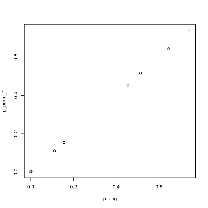
This case permutation and analytical p-values are the same.
Permutation testing scheme 2 – minimum p-value
Here we perform permutation testing on the data as follows:
- Permute the phenotype vector
- Perform association tests and get the minimum p-value among the 10 permuted tests
- Compare the minimum p-value with each of the 10 SNPs’ original p-value. If the minimum p-value is smaller than the original p-value we call it a “success” and otherwise “failure”
- Repeat 1 - 3 numerous times. Empirical p-value is defined by the total number of success divided by the total number of permutations
Let’s use 10,000 permutations for this problem:
test_perm_2 = function(X,y,K=10000) {
    p_orig = test_assoc(X,y)
    res = matrix(0, K, ncol(X))
    for (i in 1:K) {
        p_perm = test_assoc(X,sample(y))
        min_p = min(p_perm)
        res[i,] = sapply(p_orig, function(x) x>=min_p)
    }
    return(apply(res, 2, mean))
}
p_perm_2 = test_perm_2(X,y)
If this permutation scheme is correct, we would expect that it is comparable to a Bonferroni correction of testing 10 independent hypothesis
bonferroni_correct = function(p) 1 - (1 - p) ^ length(p)
bonferroni_correct(p_orig)
plot(bonferroni_correct(p_orig), p_perm_2)
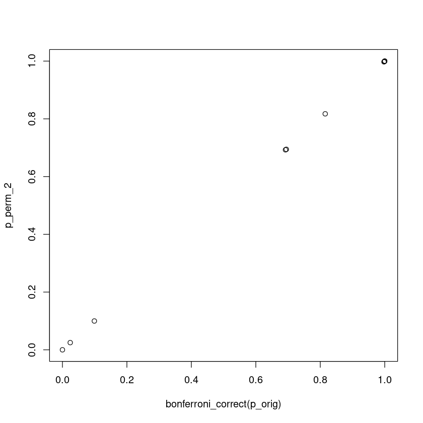
p_perm_2
The Bonferroni and this permutation theme give the same result because by definition, both Bonferroni and this permutation assess if the most significant association is real. By using the minimum p-value, permutation test gives the empirical distribution of the most extreme statistic.